The Inner Product, April 2002
Jonathan Blow (jon@number-none.com)
Last updated 17 January 2004
 

Inverse Kinematics with Quaternion Joint Limits

Related articles:

Hacking Quaternions (March 2002)
Understanding Slerp, Then Not Using It (April 2004)

This month we're going to talk about inverse kinematics ("IK"). Jeff Lander wrote a series of introductory articles about IK in 1998; see the references.

There are a few different paradigms for solving IK problems, but we're going to concentrate on Cyclic Coordinate Descent (CCD). CCD is easy to implement and is fairly modular -- you can hack stuff into it without too much trouble.


How CCD Works

CCD is an iterative numerical algorithm. You have a chain of joints, which I will call the "arm"; the arm is in some initial state, and you want the end of the chain, the "hand", to reach some target. We have some measure of the error in the current state of the arm, which involves the position and orientation of the hand with respect to the target. CCD iterates over the joints in the arm, adjusting each in isolation, with the goal of minimizing this overall error. See Figure 1.

To animate a human character, we want CCD to give us solutions that are valid for a human body. When picking a glass up from a table, we don't want the character's elbow to bend backwards in a physically impossible way. In order to prevent this, we can enforce limits on the ways each joint can bend. A shoulder has all 3 degrees of rotational freedom, but each degree is limited -- the shoulder can only reach through a certain range of angles and can only twist so far. An elbow might be modeled with 2 degrees of freedom: one that bends the forearm toward the upper arm, and another that twists the forearm.
 

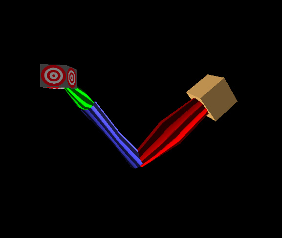
Figure 1: A 3-segment arm (anchored at the tan cube) reaching to a target (cube with target texture on it).  The arm segments are red, green, and blue.  The striped textures show the amount of twist contained within each bone transform.

CCD Convergence Issues

Because CCD is iterative, you can enforce these limits at each step just by taking the resultant orientation for any joint and forcing it to stay within the valid range. However, this affects CCD's ability to converge on an answer. CCD is a blind hillclimbing algorithm; it is walking across a terrain defined by your error function, trying to find the highest point. But when you impose joint limits, you stick invisible walls on the terrain that the hillclimber isn't aware of.  Envision a typical situation: the system is trying to reach the target by expanding the elbow beyond its joint limit; after each iteration the elbow is forced back within limits, so the algorithm doesn't get anywhere.

We can detect this situation and attempt to re-solve the system by starting the arm in a different configuration where that particular wall will no longer be in the way. This is a special case of a time-honored tool called simulated annealing.

Using the most basic form of simulated annealing, you would reset each joint to a random pose and try again. This is probably the easiest to code. A solution that may perform better at runtime is to precompute a fixed number of starting positions for the arm. During a preprocess, we can randomly choose a large number of points in space; for each target point, we discover a starting configuration for which IK is sure to converge. For experiments I've tried with reasonable arms, 4 starting positions is enough. You cluster the group of test points reachable from each starting state. At runtime, given a target in arm-relative space, find the cluster centroid that is closest to the target and use the corresponding initial state.

In this month's sample code, though, I just chose the starting points by visual inspection. I interactively moved the target around until I found a situation that caused the solver to fail. Then I would find a nearby target for which convergence was successful, and I used that successful final arm state as the initial state for the new target. This lackadaisical approach may actually be fine for most projects, because not many starting configurations are needed. (It is important to realize here that I am restarting the arm in a neutral position every frame. If you choose to begin the CCD solve from an unpredictable pose, this problem becomes harder.)


Implementing Joint Limits

So we want to write a program that does this. How do we allow the animator to express joint limits, and how do we write the code to enact those limits? We know that commercial animation packages like Maya and 3D Studio MAX will do IK; we might follow their examples. But those systems don't have very intuitive interfaces, and they don't provide good control over what the IK solver does. So we're going to roll our own.


A Nicer Rotation Decomposition

Common IK packages allow you to express joint limits by clamping Euler angles, componentwise, into adjustable intervals. But the resulting set of valid directions for the bone is kind of weird, and you have minimal control over its shape. Consequently, the IK solver comes up with solutions that you don't want, and you need to fix them up. This is tedious even in off-line animation; it's unacceptable for an interactive game. So I'm going to discuss an alternative rotation decomposition, and means for limiting rotations, that is cleaner than Euler angles.

As we discussed in the February 2002 article, any two (noncolinear) unit vectors a and b define a plane. We can construct a "simple rotation" that rotates a onto b, but does not affect vectors orthogonal to the plane. The quaternion form of this rotation is the square root of the Clifford product ab; you can compute this with a dot product, a cross product, and a little bit of trigonometry (see the Hestenes book). If we wish to limit a bone rotation R, we can factor it into two rotations: one is the simple rotation that moves the bone into its final direction vector, and one represents the twist around that final vector.

We will adopt the convention that a bone is oriented along the x axis of its local transform. We perform a CCD step that yields a rotation R for some bone, and we want to joint-limit R. Let x' = Rx, direction vector in which the bone points after rotation. We first compute S = Simple(x, x'), the simple rotation that points the bone in the same direction R does. Now let R = TS, where T is a rotation representing the discrepancy between S and R. Rx = x' implies that TSx = x', but since Sx = x', T must leave the vector x' unchanged. That is, x' is an eigenvector of T, so T is a rotation around x'. Beginner's Linear Algebra says that T = RS^-1.

Suppose we want to implement a shoulder joint, which has a limited amount of twist and a limited space into which the vector can reach. We compute T and S, then limit each of T and S separately. In this month's sample code, all rotations are represented as quaternions. To limit twist, it's a simple matter to decompose the quaternion representation of T into an axis and an angle (though we actually knew the axis already, it's x'), clamp the angle, and turn that back into a quaternion.

This decomposition is nice because it talks about rotations in terms of two concrete things that we can visualize, that are close to the things we care about for doing human body animations, and that have no hidden gotchas (or at least, none nearly so bad as the Euler angle confusions). The things we think about are, "what direction does the bone point in?" and "how twisted is it?"

The Euler angle representations used by animation packages will create twist even when they don't intend to rotate around the axis of the bone. As the angles get larger, more unintentional twist is imparted toward the extremes. Our decomposition does not have this problem.


Limiting Reach

Think of the bone we're limiting as a vector pointing out into space from the origin. We can limit the "reach window" of the bone just by defining some wire loop hung in space and declaring that the bone must always pass through that loop. The loop is embedded in a plane some distance from the origin. We can choose an arbitrary polygonal shape for the loop; then figuring out whether bone is inside it becomes a 2D point-in-polygon problem. That kind of problem is considered pretty easy these days. So we have a versatile, and easily visualizable, method of restricting where the bone can go.

To keep the implementation simple, I am only supporting convex reach windows; I don't see what we would do with something more complicated than that at the present time. If we want our joints to be able to reach beyond a single hemisphere, we can use multiple convex windows embedded in different planes. For an alternative formulation of reach windows that supports star polygons, see the JGT paper by Wilhelms and Van Gelder. They also tend to discuss a 3D "reach cone" rather than a reach window, but the ideas are equivalent. I prefer to think about this problem in 2D because they're easy to sketch on paper that way (and for other reasons that we'll see next month.)

Figure 2 shows what we do when we bang up against a reach limit. We find which side of the reach window we slammed against, and then find the closest point along that segment to the destination; that point represents our final direction. Wilhelms and Van Gelder just use the point where the bone slams into the wall (the intersection of blue and brown segments in the figure), but it seems to me that if you do this numerical algorithms like CCD will have difficulty finding the best point in the window. They would grind against the wall, moving very slowly.  On the other hand, when we use a polygonal representation for our reach cone, the closest-point solution will tend to linger in the corners of the polygon, which Wilhelms and Van Gelder's solution will not.  The choice of which method to use probably depends on your application.
 

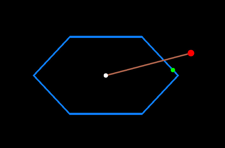Figure 2: 2D diagram of an attempted rotation that would exceed the reach window.  The blue hexagon represents the reach window; the white dot represents the endpoint of the bone when it is in the identity transformation, I.  The red dot is the endpoint of the bone after the attempted rotation which we will call R..  The brown line represents the path of interpolation between I and R.  To limit the rotation, you might think to choose the point where this interpolation path hits the wall of the reach cone (intersection of brown and blue lines).  However, this does not represent the closest valid rotation (green dot), so you may wish to solve for that instead.  However, the green dot has the property that it will linger in corners as the red dot sweeps through space, so it is not the best solution for all applications.

Tuning for Speed

Converting a rotation to the reach/twist representation is computationally cheaper than using Euler angles, but it still seems to involve some expensive operations (one _acos_ and one _sin_). But it turns out that we only need to perform this conversion if our rotation is trying to exceed the limit. We can develop quick and cheap tests to determine whether the rotation is within bounds; if it is, we just accept it and move on.

When testing reach, we just compute x' = Rx without doing the ST decomposition. If x' is within the reach window, we can exit early. Checking this still involves a point-in-polygon test, but for each reach window we can precompute the radius of a large inscribed circle, and a vector that points to the center of that circle. Then a simple dot product provides an early-accept; we only need the point-in-polygon test when x' does not pass through that circle.

This test can be even faster than we expect. Rx is much cheaper to compute than a normal quaternion-vector multiply (because two components of x are 0); but if the inscribed circle is centered around the x axis, then in the end we are computing (x . Rx), in other words, only the x coordinate of Rx. This requires only 4 multiplies and 3 adds: it is (q_w² + q_x² - q_y² - q_z²), where our rotation is the quaternion (q_x, q_y, q_z, q_w). If this quantity is greater than some precomputed constant, we know the joint's reach is safe.

This same trick can be used to accelerate the computation of the simple rotation between x and Rx (we can simplify the cross product as well as the dot product). But the trigonometry involved in taking the square root of the resulting quaternion is implicitly slow, so this optimization might seem ineffective. But the square root of some quaternion q is the point on the 4D unit sphere halfway between q and (0, 0, 0, 1). In other words, it's Slerp(1, q, 0.5). We can use our superfast quasi-slerp from last month to compute this.

But recall that 0.5 is a point of symmetry for linear interpolation -- aside from the endpoints, this is the one spot where a lerp gives you precisely the same direction as a slerp. So we can discard much of our quasi-slerp; all we need to retain is the fast normalizer. We need to modify that normalizer, though: it needs to work for lerp distortion all the way up through 180 degrees, because this is one interesting case where we are not supposed to force our quaternions into the same half-sphere before interpolating.

I present to you Listing 1, the fastest simple-rotation-finder in the West. If the two inputs to this function are x and Rx, you can further collapse the rotation, dot product, and cross product and use the CPU savings to rule the world. (A tidbit: the quaternion for any simple rotation starting from x always has an x component of 0). It is worth reiterating that Listing 1 computes exactly the right answer, to within the scale factor introduced by the normalization approximation.


Fast Twist Limit Testing

We've discussed how to quickly test for reach limits, but we can speed up twist limit testing as well, by not computing all of T. All we really need is the cosine of the twist angle, which we can test against a precomputed constant. To get this, compute Ry · Sy. We've seen in the paragraph above that S is fast to compute; Ry and Sy are again cheaper than normal quaternion-vector multiplies.



Acknowledgements

Thanks to Casey Muratori for pointing out Wilhelms and Van Gelder's JGT paper.


References

"A Combined Optimization Method for Solving the Inverse Kinematics Problem of Mechanical Manipulators," Li-Chun Tommy Wang and Chih Cheng Chen, IEEE Transactions on Robotics and Automation, Vol 7 No 4, August 1991

Clifford Algebra to Geometric Calculus: A Unified Language for Mathematics and Physics, David Hestenes and Garret Sobczyk, Kluwer Academic Publishers, 1984.

"Fast and Easy Reach-Cone Joint Limits", Jane Wilhelms and Allen Van Gelder, Journal of Graphics Tools, Volume 6 No 2, AK Peters, 2001.

Jeff Lander's Game Developer Companion source page, http://www.darwin3d.com/gdm1998.htm.

"Mathematical Growing Pains", Jonathan Blow, Game Developer Magazine, February 2002, CMP Media.