
Figure 1a: Original image of a road sign.
Figure 1b: A close-up of the corner after mipmapping via the Discrete Fourier Transform. Note the unwanted bands of color ("ringing").
The Inner Product,
January 2002
Jonathan Blow (jon@number-none.com)
Last updated 16 January 2004
Mipmapping, Part 2
Related articles:
Mipmapping, Part 1 (December 2001)
Let's continue our quest for higher-quality mipmaps. Last month we saw that Kaiser filters produce output of a fairly nice quality. According to the tenets of signal processing, the more CPU we are willing to spend, the wider we can make our filters, and the higher the output quality will be. But when we tried to make our filters very wide, we saw disturbing ripples in our output images, so we settled on a filter that was not very wide after all.
We suggested that these ripples were caused by oscillations in the frequency response of the filter. But the output ripples didn't go away even as the filters became ridiculously large and their frequency responses approached the ideal. This suggests that additional causes lurk behind the scenes. As it happens, identifying the guilty phenomena is important for our understanding of much of computer graphics, not just mipmapping.
Ditching Filters
Wide Kaiser filters are just approximations to an infinitely wide sinc pulse, which we said would remove the high frequencies from our image. Sinc does what we want because its Fourier transform is a rectangular pulse; when applied to the Fourier transform of our signal, this pulse multiplies the low frequencies by 1 and the high frequencies by 0.
In applications like live audio processing, you want to respond to a signal coming over a wire with low latency; for these cases, the filtering form of antialiasing is well-suited. But since we are mipmapping as a batch process, we have the option of just performing the Fourier transform on our texture map, manually writing zeroes to the high frequencies, and then transforming it back.
Mathematically, this is the same as filtering with an infinitely wide sinc. Since we are perfectly enacting the rectangular pulse frequency response, none of those frequency response ripples due to a finite filter can exist to cause us problems. Therefore our output will be perfect, or so we might expect.
But our output isn't perfect. The texture map still has horrible ripples in it, as you can see in Figure 1. It looks much like the output of FILTER_BAD_RINGING from last month, which was processed with a 64-sample Kaiser filter.
|
|
|
|
Figure 1a: Original image of a road sign. |
Figure 1b: A close-up of the corner after mipmapping via the Discrete Fourier Transform. Note the unwanted bands of color ("ringing"). |
Life isn't simple, so there are multiple causes for these ripples. We'll look at the two most important ones. First though, I'll mention that this month's sample code implements the Fourier transform method of mipmapping. On some images, such as the human face in the Choir Communications billboard, the results are better than the Kaiser filter. But on some other images, the results are terrible. So what's going on?
Dammit
The biggest problem is that our concept of a texture map is mathematically ill-defined. Texture maps are pictures meant to evoke in the viewer's mind the nature of the represented surface. We need to think about the mathematical consequences of the way we store texture maps, and compare that math to our mental model of the corresponding surface; we will see that the two are in conflict.
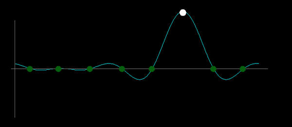
Figures 2 and 3 show a simple texture: each pixel is the same shade of green, except for one spot that is white. We interpret this as a surface that is uniformly green everywhere except in that white spot. Ideally, all the math we perform on the texture should be consistent with this mental interpretation, so that the processed image matches our expectations.
Our mental model of the image surface is a continuous function, but the texture map is not continuous; it exists only as a series of samples, which is why figure 3 is drawn the way it is.
 |
 |
| Figure 2: A solid-green texture containing a single white spot (pixels depicted as big squares). |
Figure 3: The same texture as Figure 2, drawn differently to emphasize the discrete nature of the data. |
Let's talk about sampling and reconstruction. When we sample an arbitrary (not band-limited) continuous function at 'n' points, then those points are the only information we have. In between, there could be anything at all. So suppose we take a set of samples and try to reconstruct a continuous function. We need to interpolate all the values in between, but because we threw away most of the original data, no interpolation algorithm will get us back to where we started. We just have no idea what was supposed to be between those samples.
Here's where digital filtering comes in. The Shannon Sampling Theorem is a cornerstone of information theory. It says that, if you restrict your input functions to contain only a certain range of sinusoid frequencies (the function is "band-limited"), then you can reconstruct the continuous function exactly from the samples. That's a powerful idea.
But there's a consequence to that idea. When reconstructing, we're not allowed to dictate what the function does in between the sample points; we have to take what we're given. Since the continuous function must be band-limited, it will oscillate between samples in ways that we may not expect. Figure 4 shows a 1D cross-section of our "green with white spot" texture and the continuous function it represents when we use sinusoids as our reconstruction basis. Note that the continuous version is not flat in the green area, as we would imagine it. Instead, it ripples. It can't possibly be flat, because the band-limitation constraint means that the function is unable to ease down to a slope of zero.
As far as the math we are using is concerned, here is what happened: to generate our texture, we started with some band-limited function with ripples all over the place, but when we sampled it, our sample points just happened to hit the right spots on the ripples to generate constant intensity values. Because the samples represent the entire continuous function, the ripples are still there, and our signal processing operations will reproduce them faithfully. When we shrink the texture to build mipmaps, we are essentially "zooming out" our view of the continuous function. Visible ripples appear because the change of scale and the added low-pass filtering disrupt the delicate "coincidence" of our sample point positions.
If we enlarge the source texture instead of shrinking it, we will see the ripples at our new sample points. As we move to higher and higher resolutions, we converge toward the continuous function in the limit.
Last month I mentioned that Don Mitchell, who has helped with this column by discussing many of the ideas, has a filter named after him. The Mitchell filter resulted from experiments about enlarging images without making them look icky. The Mitchell filter is intentionally imperfect from a signal reconstruction standpoint, because perfect reconstruction is not very much like what our brains are thinking about. But the Mitchell filter doesn't stray too far from the perfect upsampling either, because then nasty artifacts would appear.
In the same way that the Mitchell filter is not a perfect resolution-increasing filter, our mipmap filters, intended to decrease resolution, look best when they hover in a sweet spot between badness and goodness.
 |
 |
|
Figure 4: A 1-dimensional cross-section of the texture from figure 2, viewed from the side; the cyan curve shows the band-limited continuous function represented by these samples. |
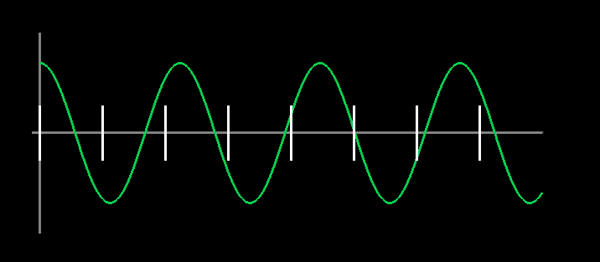
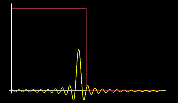
Figure 5: A low-frequency cosine wave (green) that could easily be sampled at the intervals marked in white. |
 |
|
|
Figure 6: The magnitude of the frequency content of figure 5 (graphed in yellow), as reported by the Fourier transform. It is the sum of two sinc pulses. The red step function depicts the cutoff pulse of an ideal low-pass filter. |
Do We Really Want To Antialias?
There is another important point here. The band-limited continuous-function representation, with all the unacceptable ripples, is a prerequisite to digital sampling. That is, if you walk up to a real-life green wall with a white spot on it, and you wish to create a texture map from it, then to prevent aliasing you must low-pass the incoming image before digitizing it. This filtering produces the unacceptable rippled function, and the ripples will show up in your samples. Thus digital cameras don't try to antialias this way, and they don't collect point samples to use as the photographed image. If we then treat the image as a collection of band-limited point samples, a practice which seems to be in vogue, then we introduce ripples that weren't there in the natural lightfield.
Antialiasing causes the ripples. We don't want the ripples. Therefore, antialiasing is not really what we want.
What we actually want is for all of our graphics to have infinite resolution, so that we can draw surfaces at arbitrary scales and orientations with impunity. Unfortunately, we don't yet have the means to do that, so we're using this digitally sampled image stuff instead. Antialiasing is an important tool that helps us cope with the constraints imposed by digital sampling. But it also causes some problems, so it should not be visualized as a goal in itself.
You don't generally hear that said; antialiasing is usually touted as something that only fixes problems, that has no downside. That's because an awful lot of people in computer graphics (and game programming) work from day to day using a set of concepts that they don't understand down to the core. They're just repeating what they heard from someone else, and what we get is much like the game of Telephone, where we whisper in each others' ears, and after a few transmissions the message "I biked with Pete on Friday" becomes "I'd like to eat a fried egg."
That's not to say that anyone should be blamed -- it's hard to understand all this stuff. I didn't understand it until writing this article. But there you have it: antialiasing is not really what we want. We want "elimination of objectionable artifacts", which is a different thing. Antialiasing can help in that regard, but it is not a total solution, and it can hurt too.
And that's assuming we actually know how to antialias -- which we don't. Here's why.
Questionable Interpretations
The Fourier transform is all about treating your data as a big vector and projecting it onto a set of (complex-valued) sinusoids that serve as basis functions. Each sinusoid is of a different frequency. The length of the vector in the direction of each basis function tells us something about the "frequency content" of the signal for that given frequency.
But what it tells us is not the actual frequency content. If you have a single cosine wave of the same frequency as a basis function, and you push it through the Fourier transform, you'll get what you'd expect: a single spike in the output at the appropriate frequency. But if that cosine wave has a frequency somewhere in between the basis functions, you don't get a spike any more. You get a smear of frequencies across the entire spectrum. Figures 5 and 6 illustrate this. The peak of the Fourier transformed data is in the right place, but what is going on with all that other stuff?
Even though each Fourier basis function consists of a single frequency, in the end they're still just basis functions. If you ascribe any interpretation to the transformed data, aside from "the inner product of my input data with each basis function", then you do so at your own risk. "Frequency Content of the signal" is just an interpretation, and it's a slightly misleading one.
When we low-pass filter in order to antialias, we are acting on this misleading interpretation. Consider that the cosine in figure 5 could be downsampled into a mipmap just fine, as it stands. But when we filter it, we cut off all the high frequencies to the right of the red line in figure 6. These frequencies aren't really there; when we subtract them from the cosine wave, the shape changes. We were shooting at ghosts, so we hit ourselves in the foot. This is important: some kind of imaginary "true" antialiasing would have left the cosine unscathed; but all we know is how to eliminate aliasing as the Fourier transform sees it through its own peculiar tunnel vision. This causes problems.
If we can't even antialias a dang cosine wave without messing it up, then what can we antialias, really?
Moving On
We've looked at some difficult issues underlying not only mipmapping, but many other areas of computer graphics as well (pixels on the screen are, after all, samples). It's important for engine programmers to understand these issues. But as of today there's no magic bullet for them; I can't just give you code that magically shrinks your textures while simultaneously preventing aliasing, bluring and rippling. Maybe in the future we'll have a new paradigm to help sort out these problems; maybe, if we're vigilant and our aim is true, the community of game engine scientists will develop the new concepts and techniques. Who can say?
But this is an action-oriented column, so I am obliged to provide some news you can use today. The good news is that there's something we can do, having nothing to do with choice of filter, that improves the quality of our mipmaps.
Conservation of Energy
An important goal of mipmap filters is that they don't add or subtract energy from an image; mipmap levels of a single texture should all be equally bright. This is equivalent to saying that as you sweep a filter across a given sample, the sum of all that sample's contributions does not exceed the sample's original magnitude. In other words: Σfis = s, where the fi are the filter coefficients and s is the sample value. This implies Σfi = 1: the sum of the filter's coefficients is 1.
We have a problem, though. We want the same number of photons per unit area to shoot out of the user's monitor, no matter which mipmap level we're displaying. But that doesn't happen, even though our filter's coefficients sum to 1. This is because we tend to do our image processing in a color space ramped by the monitor's gamma, which messes up the energy conservation properties.
Figures 7 and 8 demonstrate this. Figure 7 is a high-contrast texture at full resolution. Figure 8 is a lower-resolution mipmap constructed in the naive way; the areas containing fine features have gotten significantly dimmer.
 |
 |
|
Figure 7: A high-contrast texture at full resolution. |
Figure 8: The high-contrast texture reduced by 3 mipmap levels (box filter). The text has become somewhat dim, and the outlining rectangle has become extremely dim. This is energy loss due to the gamma ramp. |
Here's a quick gamma recap: Unless we do weird tweaking with our graphics card's color look up tables, the amount of light coming out of a CRT is not proportional to the frame buffer value 'p'. It is proportional to pγ, where γ (gamma) is a device-dependent value typically above 2. Our eyes interpret light energy logarithmically, so this exponential outpouring of energy looks somewhat linear by the time it gets to our brains.
We store all our texture maps in a nonlinear way -- they expect the CRT to exponentiate them in order to look right. This serves as a compression mechanism; we would need more than 8 bits per channel if each channel held values proportional to light energy.
Suppose we pass a simple box filter, coefficients [.5 .5], across a sample of magnitude 's'. We get 2 contributions to the image, of magnitude .5s and .5s. That adds up to s again, so far so good. Now the CRT raises these values to the power gamma. Now we have 2 adjacent pixels of magnitude .5γsγ. For simplicity suppose gamma is 2. Then the total amount of light energy is .25 sγ + .25 sγ = .5 sγ... but this is only half as bright as it should be (the unfiltered pixel would have output sγ). Our image got dimmer.
We can fix this by filtering in a space where pixel values are proportional to light energy. We convert our texture into this space by raising each pixel to the power γ. Then we pass our filter over the texture, ensuring conservation of energy. We then raise each pixel to the 1/γ to get back to the ramped space so we can write the texture into the frame buffer. (The CRT will raise each pixel to the gamma again during output).
It would be cleaner to set up the frame buffer so that all values stored in it are linear with light energy; the RAMDAC would perform any necessary exponentiation. High-end film and scientific rendering all happens in linear-light; game rendering will switch to this paradigm soon. When the frame buffer is linear-light, you can correctly add radiance to a surface just by adding pixel values in the frame buffer. (Right now when we shine multiple lights on a surface, we just add the values together, but the gamma ramp makes that wrong. This is one reason why lighting in PC games is dull and limp.)
This month's sample code implements mipmapping in linear-light space, and you can see the results on a game texture in figure 9.
That's all for mipmapping for now. Next month: Something else.
|
|
|
|
|
Figure 9a: A highway shield mipmapped using a typical game's box filter. |
Figure 9b: A Kaiser filter does a better job of preserving the shapes of the numbers and the sign border. |
Figure 9c: Moving the Kaiser filtering into light-linear space, we maintain the contrast between the numbers and the background, and we preserve the white border around the edge of the shield.
|
Acknowledgements
The "Phoenix 1 Mile" texture is by Dethtex [original URL no longer valid].
Thanks to Don Mitchell, Sean Barrett, and Jay Stelly for fruitful discussion.
Further Reading
Charles Poynton, "Frequently Asked Questions about Gamma". http://www.poynton.com/GammaFAQ.html
Jim Blinn, Jim Blinn's Corner: Dirty Pixels, Morgan Kaufmann Publishers.
R.W. Hamming, Digital Filters, Dover Publications.