
The Inner Product, September 2002
Jonathan Blow (jon@number-none.com)
Last updated 17 January 2004
My Friend, the Covariance Body
Related articles:
Toward Better Scripting, Part 1
(October 2002)
Toward Better Scripting, Part 2 (November 2002)
Game worlds are becoming increasingly complicated. As programmers, we write rules that determine how the game world behaves. Those rules need to produce increasingly complex results as output; as for input, they need to deal with larger volumes of world state, and the world state describing any particular entity is becoming ever more intricate.
As a result, unsurprisingly, games are becoming harder to create. One way we might cope with this is simply by becoming better, more experienced programmers. But there's a limit to how far we can push that before we snap or something, so we need other options. One option is to use ever-larger teams of programmers to create games, but it's clear from experience that that doesn't work very well.
So what can we do? We can adopt more powerful methodologies; this has benefited us greatly in the past, as we program in C++ now instead of assembly language, and we're much better for it. Unfortunately, new methods and concepts don't come along very often. So we need to actively seek them out, or invent them.
So our game worlds contain huge amounts of information, and we need to process all that stuff to produce meaningful results. I propose turning to the well-studied field of statistics to find ideas that can help us here. One of the purposes of statistics is that you can summarize large amounts of data in useful ways, and you can perform well-defined mathematical operations on that summarized data.
Statistical methods can be extremely robust in the presence of noise or incorrect inputs, where discrete algorithms would fail outright. This is important because "rigid algorithmic failures" are a big source of headache in modern games. Stochastic algorithms can provide a terrific speed boost as well; for example, Monte Carlo Ray Tracing (MCRT) and its algorithmic descendants are widely believed to be the best methods of high-end scene rendering. But game programmers' statistical tool-sets tend to be very small, so I'd like to introduce a tool that I call the "covariance body".
You can find brief presentations on the idea of covariance on random web sites, or in statistics or physics books. That material is often unfocused, difficult to wade through, or just hidden in a place where most game developers won't come across it. The purpose of this article is to present covariance bodies in a utilitarian way, and to show clearly how they can be used.
Two months ago I made a passing reference to covariance matrices, in the article about transmitting vectors over a network. I discussed the fitness of squares versus hexagons for tiling the plane, and said that covariance matrices can tell you their relative compactness. This month I'll show how.
"Covariance body" is a nonstandard term that I chose to represent a certain set of values that we can manipulate as a coherent entity. A covariance body can summarize a set of vectors in any number of dimensions; for simplicity, we'll restrict ourselves to 2D here, but the generalization is straightforward.
The quantities that make up a 2D covariance body are a 2x2 matrix, representing the covariance of the vectors; a 2-vector, the mean of the input vectors; and a scaling factor that I will call "mass", which is the sum of the masses of the input vectors. In the simplest case, the input masses will be 1, but it's often useful to weight the contribution of various vectors (for example, weighting them according to how confident you are that they belong in this particular set).
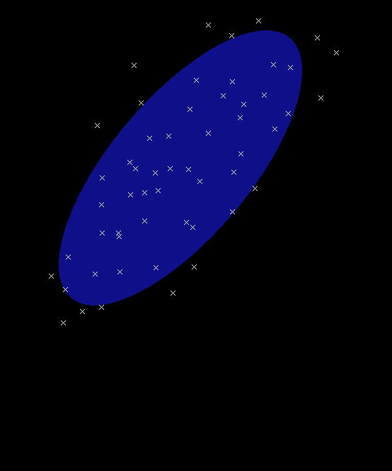
People who have done a lot of physics programming will find covariance bodies extremely familiar; they consist of the same stuff that you work with when rotating a physical body in space. This correspondence to physical bodies is nice, because when you think about what will happen when you manipulate these things, your intuition will usually be right. Mathematically, these quantities together represent an ellipse positioned in space, as shown in Figure 1.
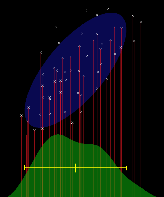
The shape of the ellipse is determined by the covariance matrix. So what is "covariance", exactly? In games we often deal with scalar time-series data, and we know that the _variance_ measures how much the input value tends to change from sample to sample. But for today's purposes, we don't want to think about it that way. We want to visualize the distribution of input values, and think of the variance as characterizing the approximate width of that distribution (Figure 2).
When you have multidimensional inputs, you can compute the variance for each dimension separately. But you can also compute the correlation between the dimensions, and that is what we mean by covariance. "Covariance matrix" is shorthand for what is also called the variance-covariance matrix, which is what you get when you stick variance and covariance together into a coherent mathematical structure.
 |
 |
| Figure 1: A set of data points and an ellipse that summarizes them. The ellipse is drawn at 1.7 standard deviations. | Figure 2: We consider the 1-dimensional statistics of the data points, by projecting them down to the X axis (projection shown by red vertical lines). The 1-dimensional distribution, drawn in green, has a mean and spread indicated by the yellow bar; the edges of the bar are at 1.7 standard deviations. These notches on the yellow bar also correspond to the center and edges of the ellipse when projected onto the axis. (Note: the distribution in green was computed by convolving a Lanczos-filtered sinc pulse with the delta function representing the presence or absence of a projected point on the X axis). |
So, you've got a bunch of input points. These could be positions in the game world, pixels in a bitmap, or whatever. Each point has associated with it a certain mass, its relative importance. The total mass of all the points is mtotal = Σmi, where mi is the mass of an individual input. The weighted mean of these points, analogous to their center of mass in the physical world, is: vcenter = mtotal-1 Σmivi, where vi is the ith position.
Let v’i be the position of a point relative to its center of mass, that is, v’i = vi - vcenter. Then the covariance matrix, which describes how mass is distributed in space around the center, is the outer product mtotal-1 Σmiv’iv’it. Expanding this product for the 2D case gives us the 2x2 symmetric matrix:

where vi = (xi, yi).
The covariance body consists of these quantities, the n × n symmetric covariance matrix C, the n × 1 vector for the center of mass x, and the scalar total mass m. Occasionally I will refer to a particular covariance body using the notation { C, x, m }.
The covariance matrix C tells us the variance of our mass as a function of direction. That is not very much information, compared to the large amount of data we started with. But it can serve as a tidy summary. We can take a simple shape that has the same variance as our input data and visualize that. Another way to think of this is that, by computing the variance of our input mass, we have least-squares fitted this simple shape to the input.
The Gaussian curve is one of the most natural shapes for talking about the distribution of mass. The Fuzzy Central Limit Theorem states that when you sum together enough arbitrary random processes, the result is a "normal distribution" (a Gaussian; See For More Information). Since most sets of data result from the interaction of a large number of random-seeming processes, the Gaussian is a good way to describe them.
The 2D version of a Gaussian is known as a Gaussian bivariate distribution; it has two variances, a maximum and minimum. The level sets of this Gaussian -- points for which the function has a constant value -- are ellipses. One way to visualize this Gaussian in 2D is to draw a characteristic ellipse.
The eigenvalues of a covariance matrix tell you the maximum and minimum variance of its Gaussian as a function of direction; you square-root the eigenvalues to get the length of each axis of the ellipse. This is because variance is computed in squared units, and you want lengths in the native units of your input; so, you want the standard deviation, which is just the square root of the variance. The square root operation won't cause any problems since the eigenvalues are guaranteed to be non-negative (though they might be zero!)
The eigenvectors of the covariance matrix tell you the direction in which each eigenvalue is achieved; this provides the ellipse's orientation. The mean tells you where the ellipse should be positioned. That's all the information you need to draw the ellipse on the screen.
One nice property of covariance bodies is that you can quickly combine two bodies A and B. The body you get as a result is the same thing you would have computed if you had re-iterated over all the input masses comprising A and B. You can speculatively combine covariance bodies in hierarchies and speedily diagnose the resulting shape. This was very useful to me in a recent image processing application, which required churning through a large number of shape combinations.
Suppose you wish to add two covariance bodies { C1, x1, m1 } and { C2, x2, m2 }. Intuitively, the mass of the resulting body is m3 = m1 + m2. It's also not difficult to figure out that the new mean is a weighted average of the old means, depending on each body's mass: x3 = (m1x1 + m2x2) / (m1 + m2). To compute C3, we need to shift C1 and C2 so that they represent each body's mass distribution with respect to the new mean. Then we can add the matrices together, and that gives us C3.
To see how to shift a covariance matrix to a new reference point, expand the expression mtotal-1 Σmi(xi + s) (xi + s)t, where s is the vector from the old reference point to the new one. Expanding this product gives you: C + sxt + xst + sst, where x was your old reference point (until now, the center of mass).
Other linear operations can be summed with similar ease. In my image processing application, I wanted to least-squares fit a set of planes to the RGB values that comprised each covariance body, so that I could later reconstruct a linear approximation to the color over the whole region. Interestingly, the math for this least-squares fit used the same covariance matrix that I was already computing; it just used it in a slightly different way, where I would solve an Ax=b problem to get the results, instead of an eigenvector problem. So the only additional information I needed to keep around was the 'b' vector for the right-hand side of this equation. When summing covariance bodies, I would just compute b3 = b1 + b2, and suddenly I had an aggregate least-squares color fit over the summed body. It was cool.
Two months ago I talked about using the hexagon versus the square to tile the plane, in order to transmit the position of an entity over the network. I said that the hexagon was a better choice, because it is more compact than the square.
Covariance provides one method for finding the compactness of a shape. In 1D, given two distributions of the same amount of mass, the distribution with the smaller standard deviation is more compact. The situation is more confusing in 2D, where a distribution can be compact in one dimension but widespread in the other. I tend to measure compactness using the average standard deviation with respect to direction, which you can find by integrating over one quarter of the ellipse:

This works out to (a + b) 2/π, where a and b are the lengths of the axes. If we only care about relative compactness, we can throw out the scaling factor and just use (a + b).
If we're dealing with shapes of constant density and area, like the square versus the hexagon, a circle represents the most compact possible shape. This is verified by our compactness measure: if Area = 2πab, then ab = k = Area / 2π, thus b = k/a; if you allow a to vary and you minimize (a + b), the answer you get is a = b = sqrt(k), a circle.
So to find the compactness of a 2D shape, we just need its covariance. You can compute the covariance for a 2D shape in closed form; just integrate the covariance matrix over each point in the shape. You can generically handle polygons, without writing a specific equation for each one; all you need is the closed form equation for the covariance of a triangle (an exercise left to the interested reader.) Then, to find the covariance of a polygon, you just triangulate it, compute the covariance body for each triangle, and combine those bodies.
This month's sample code illustrates the construction and combination of covariance bodies to summarize data. You can input a bunch of masses by clicking on the screen, and the program draws the resulting ellipse. So far this has all been a little bit divorced from the day-to-day concerns of game programming, but I'll apply covariance to a concrete and relevant topic next month, when we look at ... scripting languages.
Thanks to Charles Bloom for a discussion about the Gaussian's special role in statistics.
"Central Limit Theorem" from Eric Weisstein's World of Mathematics, http://mathworld.wolfram.com/CentralLimitTheorem.html